轻量的神经网络

很久之前我觉得移动端应用几百兆的模型不切实际，在不考虑蒸馏、量化等压缩方法下，发现了 MobileNet 设计的很神奇，大小只有几 MB，可以说是一股清流了。就整理发布了一下，然后今天发现找不到了，神奇。（于是顺手和 ShuffleNet 一并整理到轻量化的神经网络中）

MobileNet-V1

基本上可以说这个版本是后面几个版本的出发点。先来看一下创新点：提出 depthwise separable conv 和 pointwise conv 来降低网络的计算次数。还是直接画图吧：

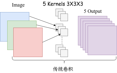
对于传统卷积而言，输入一个三通道的图片，如果想要输出五通道，那么就需要 5 个 $3\times 3 \times 3$ 的卷积核。一般一些，假设传统卷积处理图像的大小是 $D_F\times D_F$，有 $M$ 个通道，卷积核的大小是 $D_K$，输出的通道数数 $N$，那么计算量就是 $D_K \cdot D_K \cdot M \cdot N \cdot D_F \cdot D_F$。

在得到相同大小输出的情况下，使用 DW 卷积和 PW 卷积来简化一下这个计算过程：

如果换成深度可分离卷积和逐点卷积，可以看到达到同样的输出，参数量从 $27\times 5$ 减少到了 $27+15$，而且计算量为 $D_K \cdot D_K \cdot M \cdot D_F \cdot D_F + M \cdot N \cdot D_F \cdot D_F$。两者的比值是 $1/N+1/D_K^2$。

class MobileNetV1(nn.Module):
    def __init__(self, ch_in, n_classes):
        super(MobileNetV1, self).__init__()

        def conv_bn(inp, oup, stride):
            return nn.Sequential(
                nn.Conv2d(inp, oup, 3, stride, 1, bias=False),
                nn.BatchNorm2d(oup),
                nn.ReLU(inplace=True)
                )

        def conv_dw(inp, oup, stride):
            return nn.Sequential(
                # dw
                # 输入通道和输出通道相等，groups 表示每个卷积核只处理一个通道
                nn.Conv2d(inp, inp, 3, stride, 1, groups=inp, bias=False),
                nn.BatchNorm2d(inp),
                nn.ReLU(inplace=True),

                # pw
                # 卷积核大小为 1X1
                nn.Conv2d(inp, oup, 1, 1, 0, bias=False),
                nn.BatchNorm2d(oup),
                nn.ReLU(inplace=True),
                )

        self.model = nn.Sequential(
            conv_bn(ch_in, 32, 2),
            conv_dw(32, 64, 1),
            conv_dw(64, 128, 2),
            conv_dw(128, 128, 1),
            conv_dw(128, 256, 2),
            conv_dw(256, 256, 1),
            conv_dw(256, 512, 2),
            conv_dw(512, 512, 1),
            conv_dw(512, 512, 1),
            conv_dw(512, 512, 1),
            conv_dw(512, 512, 1),
            conv_dw(512, 512, 1),
            conv_dw(512, 1024, 2),
            conv_dw(1024, 1024, 1),
            nn.AdaptiveAvgPool2d(1)
        )
        self.fc = nn.Linear(1024, n_classes)

    def forward(self, x):
        x = self.model(x)
        x = x.view(-1, 1024)
        x = self.fc(x)
        return x

MobileNet-V2

V1 的思想可以概括为：首先利用 3×3 的深度可分离卷积提取特征，然后利用 1×1 的卷积来扩张通道。但是有人在实际使用的时候，发现训完之后发现 dw 卷积核有不少是空的。

作者认为这是 ReLU 激活函数导致的。于是做了一个实验，就是对一个 n 维空间中的一个东西乘以矩阵 $T$，而后做 ReLU 运算，然后利用 $T$ 的逆矩阵恢复，对比 ReLU 之后的结果与 Input 的结果相差有多大。作者发现：低维度做 ReLU 运算，很容易造成信息的丢失。而在高维度进行 ReLU 运算的话，信息的丢失则会很少。

由于卷积本身没有改变通道的能力，来的是多少通道输出就是多少通道。上面又得出低维通道不好的结论，因此使用 PW 卷积升维再降维，这也就形成了 Inverted Residuals 这种结构，因为传统的残差结构和本文相反，传统的是先降维在升维。

这样高维的仍然使用 ReLU 激活函数，低维的换成线性激活函数。因为有先升维在降维的结构，因此使用了残差连接来提升性能。

class InvertedResidual(nn.Module):
    def __init__(self, inp, oup, stride, expand_ratio):
        super(InvertedResidual, self).__init__()
        self.stride = stride
        assert stride in [1, 2]

        hidden_dim = int(inp * expand_ratio)
        self.use_res_connect = self.stride == 1 and inp == oup

        if expand_ratio == 1:
            self.conv = nn.Sequential(
                # dw
                nn.Conv2d(hidden_dim, hidden_dim, 3, stride, 1, groups=hidden_dim, bias=False),
                nn.BatchNorm2d(hidden_dim),
                nn.ReLU6(inplace=True),
                # pw-linear
                nn.Conv2d(hidden_dim, oup, 1, 1, 0, bias=False),
                nn.BatchNorm2d(oup),
            )
        else:
            self.conv = nn.Sequential(
                # pw 升维
                nn.Conv2d(inp, hidden_dim, 1, 1, 0, bias=False),
                nn.BatchNorm2d(hidden_dim),
                nn.ReLU6(inplace=True),
                # dw 深度可分离卷积
                nn.Conv2d(hidden_dim, hidden_dim, 3, stride, 1, groups=hidden_dim, bias=False),
                nn.BatchNorm2d(hidden_dim),
                nn.ReLU6(inplace=True),
                # pw-linear 激活
                nn.Conv2d(hidden_dim, oup, 1, 1, 0, bias=False),
                nn.BatchNorm2d(oup),
            )

    def forward(self, x):
        if self.use_res_connect:
            return x + self.conv(x)
        else:
            return self.conv(x)

MobileNet-V3

主要做了两点创新，一个是在 MobileNet V2 残差分支加入了 SE（Squeeze-and-Excitation） 注意力机制的模块，一个是更新了激活函数。SE 注意力就是通过池化得到每个通道的值，并输入到全连接层学习到每个通道的权重，对每个通道的数值进行更新。

class SELayer(nn.Module):
    def __init__(self, channel, reduction=4):
        super(SELayer, self).__init__()
        self.avg_pool = nn.AdaptiveAvgPool2d(1)
        # 输入维度和输出维度相同
        self.fc = nn.Sequential(
            nn.Linear(channel, _make_divisible(channel // reduction, 8)),
            nn.ReLU(inplace=True),
            nn.Linear(_make_divisible(channel // reduction, 8), channel),
            h_sigmoid()
        )

    def forward(self, x):
        b, c, _, _ = x.size()
        y = self.avg_pool(x).view(b, c)
        y = self.fc(y).view(b, c, 1, 1)
        # y 是每个通道的权重
        return x * y

在重新设计激活函数方面，使用 h-swish 激活函数代替了 swish 激活函数，因为更容易计算。对于 swish 激活函数：

\begin{equation}
\begin{aligned}
\text{swish} x &= x \cdot \sigma(x) \\
\sigma(x) &= \frac{1}{1+e^{-x}}
\end{aligned}
\end{equation}

这个反向传播和激活的计算过程略显复杂，对量化不够友好。于是使用较为接近的 h-swish 激活函数代替：

\begin{equation}
\begin{aligned}
\text{h-sigmoid} &= \frac{\text{ReLU6}(x+3)}{6} \\
\text{h-swish} &= x \cdot \text{h-sigmoid}
\end{aligned}
\end{equation}

class h_sigmoid(nn.Module):
    def __init__(self, inplace=True):
        super(h_sigmoid, self).__init__()
        self.relu = nn.ReLU6(inplace=inplace)

    def forward(self, x):
        return self.relu(x + 3) / 6


class h_swish(nn.Module):
    def __init__(self, inplace=True):
        super(h_swish, self).__init__()
        self.sigmoid = h_sigmoid(inplace=inplace)

    def forward(self, x):
        return x * self.sigmoid(x)

class InvertedResidual(nn.Module):
    def __init__(self, inp, hidden_dim, oup, kernel_size, stride, use_se, use_hs):
        super(InvertedResidual, self).__init__()
        assert stride in [1, 2]

        self.identity = stride == 1 and inp == oup

        if inp == hidden_dim:
            self.conv = nn.Sequential(
                # dw
                nn.Conv2d(hidden_dim, hidden_dim, kernel_size, stride, (kernel_size - 1) // 2, groups=hidden_dim, bias=False),
                nn.BatchNorm2d(hidden_dim),
                h_swish() if use_hs else nn.ReLU(inplace=True),
                # Squeeze-and-Excite
                SELayer(hidden_dim) if use_se else nn.Identity(),
                # pw-linear
                nn.Conv2d(hidden_dim, oup, 1, 1, 0, bias=False),
                nn.BatchNorm2d(oup),
            )
        else:
            self.conv = nn.Sequential(
                # pw 升维
                nn.Conv2d(inp, hidden_dim, 1, 1, 0, bias=False),
                nn.BatchNorm2d(hidden_dim),
                h_swish() if use_hs else nn.ReLU(inplace=True),
                # dw 提取特征
                nn.Conv2d(hidden_dim, hidden_dim, kernel_size, stride, (kernel_size - 1) // 2, groups=hidden_dim, bias=False),
                nn.BatchNorm2d(hidden_dim),
                # Squeeze-and-Excite
                SELayer(hidden_dim) if use_se else nn.Identity(),
                h_swish() if use_hs else nn.ReLU(inplace=True),
                # pw-linear 先行激活，降维
                nn.Conv2d(hidden_dim, oup, 1, 1, 0, bias=False),
                nn.BatchNorm2d(oup),
            )

    def forward(self, x):
        if self.identity:
            return x + self.conv(x)
        else:
            return self.conv(x)

ShuffleNet-V1

group 卷积能有效的减少卷积参数。假设输入图像的大小为 $c_1\times H \times W$，卷积核大小为 $c_1 \times h \times w$，想要得到 $c_2 \times H \times W$ 的输出目标，那么需要的卷积层参数量就是：$c_2 \times c_1 \times h \times w$。

如果使用 group 卷积，将通道分成 $g$ 组，那么每个输入就是 $c_1/g \times H \times W$，对应的卷积核大小为 $c_1/g \times h \times w$，为了得到同样大小的输出，一组卷积的输出大小就是 $c_2/g \times H \times W$，将 $g$ 组卷积核的输出拼接到一起得到同等大小的输出 $c_2 \times H \times W$，此时的参数量为 $c_2 \times c_1 / g\times h \times w$。

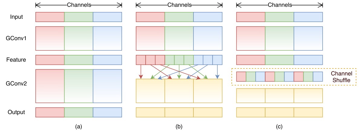
• 图 a 中，对于 group 卷积而言，channel 特征只在组内传递
• 图 b 中，对 channel 进行打乱，特征在多个 channel 中传递

综上，使用 group 卷积替换传统卷积，并在 group 卷积后使用 channel shuffle 操作。

def channel_shuffle(x, groups):
    batchsize, num_channels, height, width = x.data.size()

    channels_per_group = num_channels // groups
    
    # reshape
    x = x.view(batchsize, groups, 
        channels_per_group, height, width)

    # 通道那个矩阵发生了转置
    # - contiguous() required if transpose() is used before view()
    x = torch.transpose(x, 1, 2).contiguous()

    # flatten
    x = x.view(batchsize, -1, height, width)

    return x

ShuffleNet-V2

在众多影响模型推理速度的因素中，理论计算量只是一部分，额外的还有内存访问（memory access cost, MAC）、平台架构和并行等级；而 数据 IO、逐元素运算也会占用时间。因此作者给出了设计轻量网络的四条准则和实验验证：

\begin{equation}
\begin{aligned}
\text{MAC} &= hw(c_1+c_2)+c_1c_2 \\
{ } & \geq 2hw\sqrt{c_1c_2}+c_1c_2\\
{ } & \geq 2\sqrt{hwB} + \frac{B}{hw}\\
B &= hwc_1c_2 (\text{FLOPs})
\end{aligned}
\end{equation}

1. 如上的 MAC 计算中，可以发现当 $c_1=c_2$ 的时候取等号。也就是当卷积的输入和输出 channel 相等时，内存访问代价最低，因此尽可能使通道不变

\begin{equation}
\begin{aligned}
\text{Group-MAC} &= hw(c_1+c_2)+c_1c_2/g \\
{ } &=hwc_1 + \frac{Bg}{c_1} + \frac{B}{hw}\\
B &= hwc_1c_2/g (\text{FLOPs})
\end{aligned}
\end{equation}

1. 在 Group-MAC 计算中，因为其他是定植，那么大小取决于 $g$，因此分组卷积分的越多时，内存访问代价会增大
2. 网络的碎片化程度越高（分支越多的意思），速度越慢。对于 GPU 的并行计算不友好，而且涉及不同分支的同步问题
3. 逐元素相加也会带来不可忽视的开销，如 relu，残差的 add 运算

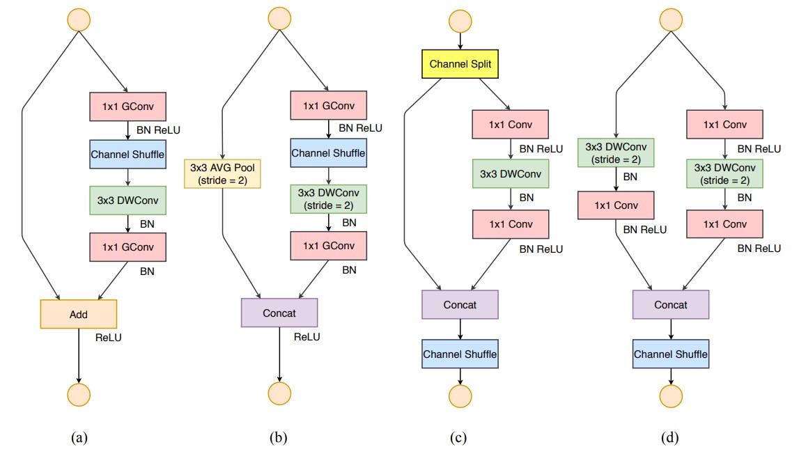
图左侧的 a（stride=1） 和 b（stride=2） 是 ShuffleNetV1 的结构，右侧的 c（stride=1） 和 d（stride=2） 是 ShuffleNetV2 的结构。

图 c 中，为了减少碎片化，在 c 中取消了左侧分支没有运算，右侧分支满足第一个准则，而最开始的 channel split 到最后的 concat，再次满足第一个准则，不选择 add 操作满足第 4 个准则。只对右侧的分支进行 relu 激活，并取消最终输出的 relu，满足第 4 个准则。而 concat，channel shuffle 和下一层输入的 channel split 可以合并为一个逐元素操作，不得不说太细了。

然后 ShuffleNetV2+ 在借鉴 MobileNetV3 的想法，也使用了 h-swish 激活函数和 SE 注意力机制，结果上超过了 MobileNetV3，这一部分可以在旷视的 github 上找到。