本来是被老师安排了写毕业论文的,但是歪打正着发现了个有趣的东西,决定先更新一下再去写(毕竟谁闲的没事想写那两万字的论文)。
通过两个新旧CPU的对比分析算法时间复杂度的重要性;
以顺序结构实现 插入排序 算法(非正解),时间复杂度$O(n^3)$;
以链式结构(双向链表)实现 插入排序 算法,时间复杂度$O(n^2)$;
对比两者,分析时间复杂度的影响。
首先,默认本文的读者有数据结构的基础,或者从任何一本《数据结构》教材里寻找:时间复杂度、插入排序、双向链表的定义。对于外行人(数据结构基础四舍五入等于没有或者只想来看热闹),可以选择只看本文你能看懂得部分,同样很有意思。
时间复杂度 参考任何一本《数据结构》的教材都能得到时间复杂度、空间复杂度的详细定义,这里不再解释。
那么,不如深刻来了解下算法复杂度对时间的影响。假设有两块CPU,第一块破旧的CPU为A,第二块CPU为B,B的性能比A好上10倍,这里假设为:B的计算速度是A的10倍。假设A计算规模为$N$的问题所需时间为$t$,理想情况下不难得到以下表格:
问题规模
CPU: A执行时间
CPU: B执行时间
$N$
$t$
$t/10$
$N^2$
$t^2$
$t^2/10$
那么对于同一个问题涉及了两种算法,第一种算法的时间复杂度为$O(n^2)$,而经过优化的算法的时间复杂度为$O(n)$,降低了一个数量级。那么,优化好的算法$O(n)$在CPU A上执行的时间为$t$,而另一个人感觉自己CPU很好没必要优化算法,那么没优化的算法$O(n^2)$在CPU B上执行的时间为$t^2/10$,设函数$g(t)$为$g(t)=t-t^2/10$,可以知道$g(t)$是开口向下的二次函数,也不难求出函数$g(t)$的两个根为$0, 10$。
当问题规模逐渐增加,问题逐步复杂,处理数据逐步增多时,即$n>10$时,函数$g(t)<0$,意味着优化过的算法在破旧的CPU A上的执行时间,要远小于性能好上十倍的CPU B。这里可以体现算法的时间复杂度的重要性。好的算法胜过好的处理器。所以,要想设计一款好软件,算法是必不可缺的功底,所以,只要还在计算机这个圈子里,数据结构就是逃不掉的。
况且在技术飞速发展的今天,硬盘空间显得不在像当初那么昂亏,可以花很便宜的价格买到容量几百个G的硬盘。所以,在不要求存储空间的问题中,可以放肆的使用硬盘空间来提升算法执行时间的效率,如:哈希算法、虚拟内存等技术,所以,一般情况下空间复杂度显得不是很重要。
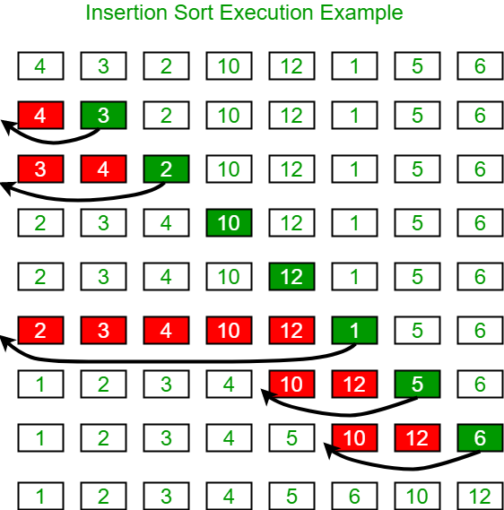
插入排序 通过一个图片简单的理解插入排序:遍历数组,把当前元素移动到合适位置即可。
顺序结构实现 正解 以下是顺序结构实现插入排序算法正解的核心代码,时间复杂度不难看出为$O(n^2)$:
1
2
3
4
5
6
7
8
9
for (int i = 1 ; i < len; i++){ int key = arr[i]; int j = i - 1 ; while ((j >= 0 ) && (key < arr[j])){ arr[j+1 ] = arr[j]; j--; } arr[j+1 ] = key; }
错解 错解的意思是:代码实现的逻辑不好,但是代码执行的结果是对的。
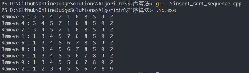
一个人编程水平不咋地,如我(我是真的写错了),我用一种错误的逻辑写出了顺序结构的插入排序代码,时间复杂度为$O(n^3)$,对序列3, 5, 4, 7, 1, 6, 8, 5, 9, 2进行插入排序,好在得到了正确的结果。如本文开头所说,本文的内容纯属歪打正着,所以之后会使用如下的错解代码,得到另外的有趣的东西。
1 2 3 4 5 6 7 8 9 10 11 12 13 14 15 16 17 18 19 20 21 22 23 24 25 26 27 28 29 30 31 32 33 34 35 36 37 38 39 40 41 42 #include <iostream> #include <fstream> using namespace std;int main (int argc, char const *argv[]) int len = 10 ; int arr[10 ] = {3 , 5 , 4 , 7 , 1 , 6 , 8 , 5 , 9 , 2 }; int temp; for (int i = 1 ; i < len; i++) { cout << "Remove " << arr[i] << " : " ; if (arr[i] >= arr[i - 1 ]){ for (int j = 0 ; j < len; j++) cout << arr[j] << " " ; cout << endl; continue ; } else { temp = arr[i]; int k = i; for (int j = i - 1 ; j >= 0 ; j--){ if (arr[j] <= arr[i] || (j == 0 && arr[j] > arr[i])){ if (j == 0 && arr[j] > arr[i]) j = -1 ; while (k > j + 1 ){ arr[k] = arr[k - 1 ]; k--; } arr[j + 1 ] = temp; break ; } } } for (int j = 0 ; j < len; j++) cout << arr[j] << " " ; cout << endl; } return 0 ; }
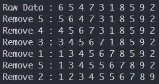
链式结构实现 因为在插入的过程中会访问当前元素之前的元素,所以有必要使用双向链表(任何一本《数据结构》的教材都能得到双向链表的定义,这里不在解释)。移动元素仔细分析指针该如何移动即可。对序列3, 5, 4, 7, 1, 6, 8, 5, 9, 2进行插入排序,不难看出我实现的代码的时间复杂度为$O(n)$。指针恐惧者慎用链式结构。
1 2 3 4 5 6 7 8 9 10 11 12 13 14 15 16 17 18 19 20 21 22 23 24 25 26 27 28 29 30 31 32 33 34 35 36 37 38 39 40 41 42 43 44 45 46 47 48 49 50 51 52 53 54 55 56 57 58 59 60 61 62 63 64 65 66 67 68 69 70 71 72 73 74 75 76 77 78 79 80 81 82 83 84 85 86 87 88 89 90 91 92 93 94 95 96 97 98 99 100 101 102 103 104 105 106 107 108 109 110 111 112 113 114 115 116 117 118 119 120 121 122 123 124 125 126 127 128 129 #include <iostream> using namespace std;struct node { node *pre; int data; node *next; }; struct head { node *first; int len = 0 ; }; int main (int argc, char const *argv[]) int arr[10 ] = {6 , 5 , 4 , 7 , 3 , 1 , 8 , 5 , 9 , 2 }; int len = 10 ; node ans[len]; head L; for (int i = 0 ; i < len; i++) { ans[i].data = arr[i]; if (i == 0 ) { L.first = &ans[i]; ans[i].next = &ans[i + 1 ]; } else if (i == len - 1 ) { ans[i].pre = &ans[i - 1 ]; ans[i].next = NULL ; } else { ans[i].pre = &ans[i - 1 ]; ans[i].next = &ans[i + 1 ]; } L.len++; } cout << "The length of link is : " << L.len << endl; node *p; p = L.first; cout << endl << "Raw Data : " ; while (p != NULL ) { cout << (*p).data << " " ; p = (*p).next; } cout << endl; p = L.first; p = (*p).next; node *s, *t; while (p != NULL ) { if ((*p).data < (*(*p).pre).data) { node *q; q = L.first; while ((*q).data <= (*p).data) q = (*q).next; if ((*p).next == NULL && q == L.first) { s = (*p).pre; (*p).next = L.first; (*q).pre = p; (*(*p).pre).next = NULL ; (*p).pre = NULL ; L.first = p; } else if ((*p).next == NULL && q != L.first) { s = (*p).pre; (*(*p).pre).next = NULL ; (*p).pre = (*q).pre; (*(*q).pre).next = p; (*p).next = q; (*q).pre = p; } else if (q == L.first && (*p).next != NULL ) { s = (*p).next; (*(*p).pre).next = (*p).next; (*(*p).next).pre = (*p).pre; (*p).next = q; (*q).pre = p; (*p).pre = NULL ; L.first = p; } else if (q != L.first && (*p).next != NULL ) { s = (*p).next; (*(*p).next).pre = (*p).pre; (*(*p).pre).next = (*p).next; (*p).next = q; (*p).pre = (*q).pre; (*(*q).pre).next = p; (*q).pre = p; } cout << "Remove " << (*p).data << " :" ; p = s; t = L.first; while (t != NULL ) { cout << " " << (*t).data; t = (*t).next; } cout << endl; } else p = (*p).next; } return 0 ; }
对比 此时,我想起了上《算法设计》这门课老师很爱干的事情,实现一个xxx算法,然后分别读入:十万、百万的数据,记录算法执行时间,对比结果。那么,既然我都写错顺序结构实现插入排序的代码了,不如歪打正着,正好对比下$O(n^3)$的算法和$O(n^2)$的算法差异。
首先用python(别问,问就是不会C++)产生随机整数,规模分别为10万,11万,15万,20万,30万,将结果保存至txt文件中。1 2 3 4 5 6 import numpy as npa = np.random.randint(0 , 500000 , 500000 ) np.savetxt('Five_hundred_thousand.txt' , a, fmt='%d' )
之后,在C++内读取文件数据,并对排序部分进行计时,顺序结构代表了$O(n^3)$的算法,链式结构代表了$O(n^2)$的算法,修改后的代码如下:
顺序结构计时 1 2 3 4 5 6 7 8 9 10 11 12 13 14 15 16 17 18 19 20 21 22 23 24 25 26 27 28 29 30 31 32 33 34 35 36 37 38 39 40 41 42 43 44 45 46 47 48 49 50 51 52 53 54 55 56 57 58 59 60 61 62 63 64 65 66 67 68 69 70 71 #include <iostream> #include <fstream> #include <ctime> using namespace std;int arr[1000002 ] = {0 };int main (int argc, char const *argv[]) int len = 0 ; string path = "Five_hundred_thousand.txt" ; string out = "Five_hundred_thousand_seq.txt" ; ifstream in (path.c_str()) ; ofstream ou (out.c_str()) ; if (!in.is_open ()) { cerr << "open file failed!" << endl; exit (-1 ); } if (!ou.is_open ()) { cerr << "create file failed!" << endl; exit (-1 ); } int a = 0 ; while (in >> a) arr[len++] = a; int temp; clock_t start = clock (); for (int i = 1 ; i < len; i++) { if (arr[i] >= arr[i - 1 ]){ continue ; } else { temp = arr[i]; int k = i; for (int j = i - 1 ; j >= 0 ; j--){ if (arr[j] <= arr[i] || (j == 0 && arr[j] > arr[i])){ if (j == 0 && arr[j] > arr[i]) j = -1 ; while (k > j + 1 ){ arr[k] = arr[k - 1 ]; k--; } arr[j + 1 ] = temp; break ; } } } } clock_t end = clock (); cout << (double )(end - start) / CLOCKS_PER_SEC << " seconds" << endl; in.close (); for (int i = 0 ; i < len; i++) ou << arr[i] << endl; ou.close (); return 0 ; }
链式结构计时 1 2 3 4 5 6 7 8 9 10 11 12 13 14 15 16 17 18 19 20 21 22 23 24 25 26 27 28 29 30 31 32 33 34 35 36 37 38 39 40 41 42 43 44 45 46 47 48 49 50 51 52 53 54 55 56 57 58 59 60 61 62 63 64 65 66 67 68 69 70 71 72 73 74 75 76 77 78 79 80 81 82 83 84 85 86 87 88 89 90 91 92 93 94 95 96 97 98 99 100 101 102 103 104 105 106 107 108 109 110 111 112 113 114 115 116 117 118 119 120 121 122 123 124 125 126 127 128 129 130 131 132 133 134 135 136 137 138 139 140 141 142 143 144 145 146 147 #include <iostream> #include <fstream> #include <ctime> using namespace std;struct node { node *pre; int data; node *next; }; struct head { node *first; int len = 0 ; }; int arr[1000002 ] = {0 };node ans[300002 ]; int main (int argc, char const *argv[]) int len = 0 ; string path = "one_hundred_thousand.txt" ; string out = "one_hundred_thousand_link.txt" ; ifstream in (path.c_str()) ; ofstream ou (out.c_str()) ; if (!in.is_open ()) { cerr << "open file failed!" << endl; exit (-1 ); } if (!ou.is_open ()) { cerr << "create file failed!" << endl; exit (-1 ); } int a = 0 ; while (in >> a) arr[len++] = a; head L; for (int i = 0 ; i < len; i++) { ans[i].data = arr[i]; if (i == 0 ) { L.first = &ans[i]; ans[i].next = &ans[i + 1 ]; } else if (i == len - 1 ) { ans[i].pre = &ans[i - 1 ]; ans[i].next = NULL ; } else { ans[i].pre = &ans[i - 1 ]; ans[i].next = &ans[i + 1 ]; } L.len++; } node *p; p = L.first; p = (*p).next; node *s; clock_t start = clock (); while (p != NULL ) { if ((*p).data < (*(*p).pre).data) { node *q; q = L.first; while ((*q).data <= (*p).data) q = (*q).next; if ((*p).next == NULL && q == L.first) { s = (*p).pre; (*p).next = L.first; (*q).pre = p; (*(*p).pre).next = NULL ; (*p).pre = NULL ; L.first = p; } else if ((*p).next == NULL && q != L.first) { s = (*p).pre; (*(*p).pre).next = NULL ; (*p).pre = (*q).pre; (*(*q).pre).next = p; (*p).next = q; (*q).pre = p; } else if (q == L.first && (*p).next != NULL ) { s = (*p).next; (*(*p).pre).next = (*p).next; (*(*p).next).pre = (*p).pre; (*p).next = q; (*q).pre = p; (*p).pre = NULL ; L.first = p; } else if (q != L.first && (*p).next != NULL ) { s = (*p).next; (*(*p).next).pre = (*p).pre; (*(*p).pre).next = (*p).next; (*p).next = q; (*p).pre = (*q).pre; (*(*q).pre).next = p; (*q).pre = p; } p = s; } else p = (*p).next; } clock_t end = clock (); cout << (double )(end - start) / CLOCKS_PER_SEC << " seconds" << endl; in.close (); p = L.first; while (p != NULL ) { ou << (*p).data << endl; p = (*p).next; } ou.close (); return 0 ; }
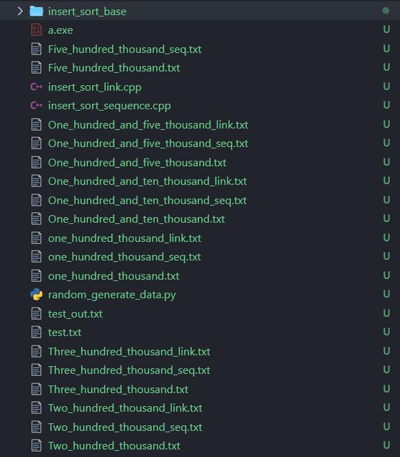
结果 文档结构如下:(每个数据规模产生一个txt文件,用于读取,输出结果加seq或者link的后缀保存到txt文件中,用于检查排序是否正确,事实证明结果是正确的,尽管代码逻辑不好,但能保证执行结果对)
在i7-9750H的CPU上执行结果如下:(执行三次,取平均)
数据规模
链式结构计时,单位:秒
顺序结构计时,单位:秒
10万
24.7
8.477
11万
30.8
10.247
15万
62
19
20万
116.112
33.765
30万
272
75.5
也许你会感到意外,为何$O(n^2)$的算法比$O(n^3)$的算法还要慢?不是不符合前文的规律?显然,这里$O(n^2)$的算法比$O(n^3)$的算法慢的原因是:链式结构要经常操作指针,来寻找下一个地址,时间耗费在地址空间的寻找上;而顺序结构中,逻辑相邻即物理相邻,不用浪费多余的时间去寻找下一个元素的地址,使用下标访问即可。
那么,如何证明前文的思想是对的?我本来是想用三次函数拟合顺序结构的数据,用二次函数拟合链式结构的数据,求两个函数的交点。结果发现数据量太少,居然只能拟合出开口向下的二次函数和单调递减的三次函数,这显然是不对的,因为这两个函数都在随着问题规模的增加,耗时逐步减少。
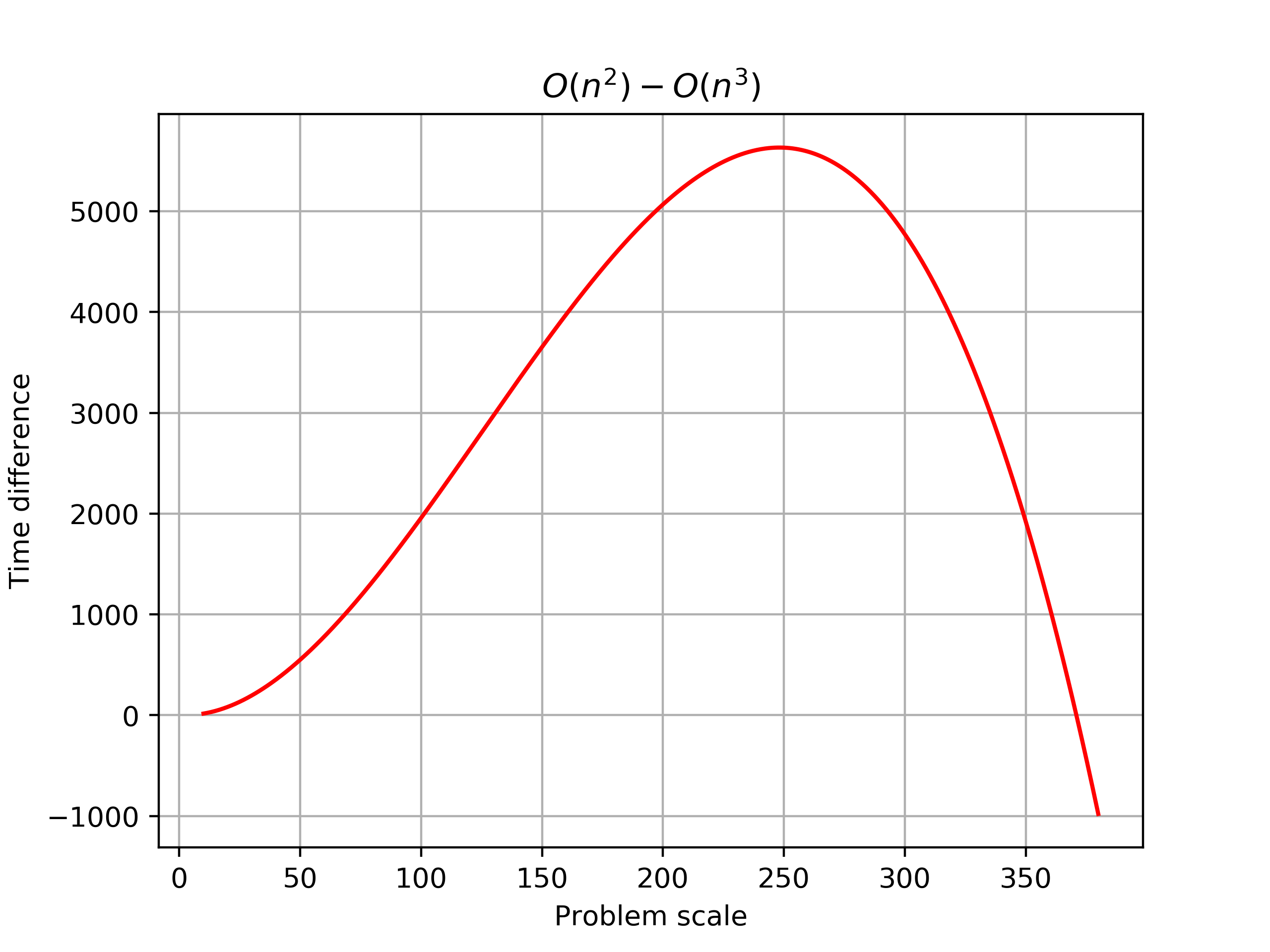
然而我还不想做更多的数据,拟合不对并不代表数据是错误的,所以,我决定用链式结构的时间减去顺序结构的时间,得到一个时间差。对时间差进行三次函数拟合(三次函数减二次函数仍然为三次函数),得到拟合结果:$g(t)=-0.0007601 x^3 + 0.2858 x^2 - 1.431 x + 2.719$,通过sympy求解,得到一个实数根为$370.95$,绘制$[10, 380]$区间内的函数图像:
可以发现,在$n>371$后,函数值小于0,说明在问题规模大于某个阈值后,$O(n^2)$的算法比$O(n^3)$的算法耗时要少,速度要快。那么这个时候,不管操作指针寻找地址多么的麻烦,时间开销总会比$O(n^3)$的算法小,只是前期可能会因为操作指针的关系影响执行的效率。
当然实际情况中,371并不代表三千多万的数据,毕竟实际情况会比单独的数据排序复杂得多。所以,也有必要根据实际问题的规模,合理的选择算法。
程序下载 下载 。我把全部文件,包括原始的随机数据、排列好的数据都放上了,后缀为seq表示顺序结构排列的结果,后缀为link表示为链式结构排列的结果。第一是证明我写的代码是对的,第二是预留这些数据,供后来者玩耍。
参考 https://www.geeksforgeeks.org/insertion-sort/